Excel Pivot Tables: From Raw Data to Summary in Minutes

A pivot table turns a long list of transactions into a clear summary in a few clicks: totals by region, counts by month, averages by product. You do not need formulas, and if you want to look at the data a different way, you simply drag a field to a new position. For anyone who works with spreadsheets, it is one of the highest-value features to learn.

This guide takes you from raw data to a useful summary step by step. It covers preparing your data, creating the pivot table, the four areas (Rows, Columns, Values, Filters), changing how values are calculated, grouping dates, showing percentages, slicers, refreshing and the mistakes that make pivot tables give wrong answers. Instructions are for Excel for Microsoft 365 on Windows; menu names are very similar in Excel 2021 and on Mac.

Step 1: Prepare the data properly

Most pivot table problems are really data problems. Before you begin, make sure your data is in a tidy, list-like format:

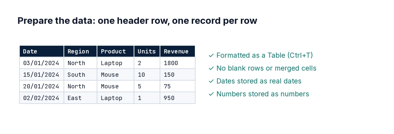
The shape of data that makes pivot tables reliable.

One header row, with a unique, non-blank name for every column.
One row per record (for example, one row per order line).
No blank rows or columns in the middle, and no subtotal rows.
Each column holds one type of data: dates are real dates, numbers are real numbers.
No merged cells.

Type this sample into A1:F13 of a new sheet (or create your own similar list):

Date        Region  Rep     Product   Units  Revenue
05/01/2024  North   Aisha   Chairs    4      480
09/01/2024  South   Ben     Desks     2      700
14/01/2024  North   Aisha   Desks     1      350
22/01/2024  East    Chen    Chairs    6      720
03/02/2024  South   Ben     Lamps     10     250
11/02/2024  North   Dev     Chairs    3      360
19/02/2024  East    Chen    Desks     2      700
27/02/2024  South   Ella    Chairs    5      600
04/03/2024  North   Dev     Lamps     8      200
12/03/2024  East    Chen    Lamps     12     300
21/03/2024  South   Ella    Desks     3      1050
29/03/2024  North   Aisha   Chairs    2      240

Then click any cell in the data and press Ctrl+T to turn it into an Excel Table. Tick “My table has headers”. Using a Table means that when you add new rows later, the pivot table picks them up on refresh. Without a Table, new rows below the original range are ignored – a very common reason for totals that do not match.

Step 2: Insert the pivot table

Click any cell inside your Table.
Go to Insert > PivotTable (in some versions, Insert > PivotTable > From Table/Range).
Check that the table name is shown as the source, choose New Worksheet and click OK.

You will see an empty pivot table on the left and the PivotTable Fields pane on the right. The top of the pane lists your column headers; the bottom shows four boxes: Filters, Columns, Rows and Values.

Step 3: Understand the four areas

Rows – the categories listed down the left side, such as Region.
Columns – categories across the top, such as Product.
Values – the numbers being summarised, such as the sum of Revenue.
Filters – a drop-down above the table that filters the whole pivot, such as one Rep.

Drag Region to Rows and Revenue to Values. You immediately get total revenue per region: East 1,720, North 1,630 and South 2,600, with a grand total of 5,950.

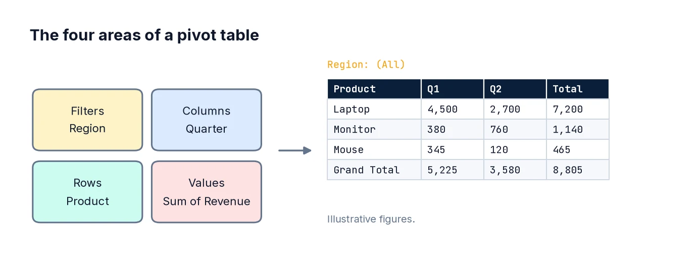
Where each field goes and how it shapes the finished pivot table (illustrative figures).

Now drag Product to Columns. You have a cross-tabulation of revenue by region and product, with row and column totals – the kind of table that would take a dozen SUMIFS formulas to build by hand.

Step 4: Change the calculation

Numeric fields default to Sum. If a numeric column contains any blank or text cells, Excel defaults to Count instead, which is a useful warning sign that your data needs cleaning.

To change the calculation, click the field in the Values box, choose Value Field Settings and pick from Sum, Count, Average, Max, Min and others. Try adding Revenue to Values a second time and setting it to Average: you now see total and average revenue side by side.

While you are in Value Field Settings, click Number Format and choose Currency or Number with a thousands separator. Formatting through the field settings sticks when the pivot table is refreshed or rearranged; formatting the cells directly often does not.

Step 5: Group dates by month or quarter

Remove Product from Columns and drag Date to Rows above Region. Recent versions of Excel often group dates automatically into Years, Quarters and Months. If not, or to change the grouping, right-click any date in the pivot table, choose Group, and select Months and Years. Always include Years if your data spans more than one year, otherwise January 2023 and January 2024 are added together.

If the Group option is greyed out or gives the error “Cannot group that selection”, at least one value in the Date column is text or blank rather than a real date. Fix the source data and refresh.

Step 6: Show values as percentages

Raw totals are not always the most useful view. Click Revenue in the Values box, choose Value Field Settings > Show Values As, and pick an option:

% of Grand Total – each cell’s share of everything.
% of Column Total or % of Row Total – the mix within each column or row.
Difference From or % Difference From – change against a previous month, for example.
Running Total In – a cumulative total, useful for year-to-date figures.

With Region in Rows and % of Grand Total applied, South shows about 43.7%, East 28.9% and North 27.4%.

Step 7: Sort and filter

To rank regions by revenue, right-click a revenue value and choose Sort > Sort Largest to Smallest. To show only the top items, click the drop-down arrow on the Row Labels header and choose Value Filters > Top 10, where you can set any number. Label filters let you include or exclude specific items.

Drag Rep to the Filters area to add a report-level filter, so you can view the whole table for one person at a time.

Step 8: Add slicers for easy filtering

Slicers are clickable filter buttons, much friendlier than drop-downs for people who read your report. Click inside the pivot table, go to PivotTable Analyze > Insert Slicer, tick Product and click OK. Clicking a button filters the pivot table; hold Ctrl to choose several. A Timeline (next to Insert Slicer) does the same for dates.

Step 9: Refresh after the data changes

Pivot tables do not update automatically when the source data changes. Add a new row to your Table, then right-click the pivot table and choose Refresh, or use Data > Refresh All (Ctrl+Alt+F5) to refresh every pivot table in the workbook. You can also set a pivot table to refresh when the file opens via PivotTable Options > Data.

Step 10: Use GETPIVOTDATA carefully

If you type = and click a cell inside a pivot table, Excel inserts a GETPIVOTDATA formula rather than a simple cell reference, for example:

=GETPIVOTDATA("Revenue", $A$3, "Region", "South")

This is actually robust: it keeps returning South’s revenue even if the layout changes. If you prefer plain references, turn it off under PivotTable Analyze > Options > Generate GetPivotData.

Common mistakes

Not using a Table as the source, so new rows are left out.
Forgetting to refresh. The pivot table shows a snapshot until you refresh it.
Numbers stored as text, which leads to Count instead of Sum.
Dates stored as text, which prevents grouping.
Blank or duplicate headers, which stop the pivot table being created.
Including total rows in the source data, which double-counts everything.
Averaging an average. If your source contains pre-calculated averages, the pivot’s average of them is not the true overall average.
Grouping months without years across multi-year data.

FAQ

Can a pivot table combine several tables?

Yes, using the Data Model. Tick “Add this data to the Data Model” when inserting, then create relationships between tables. This is the same engine used by Power BI – see Building Your First Power BI Dashboard and DAX Measures for Beginners.

How do I count unique values?

Add the data to the Data Model when creating the pivot table; Distinct Count then appears in Value Field Settings.

How do I add a calculated field?

Use PivotTable Analyze > Fields, Items & Sets > Calculated Field, for example =Revenue/Units for average price. Calculated fields work on sums, so check the results make sense.

What is the equivalent in Python or SQL?

In pandas, pivot_table or groupby (guide); in SQL, GROUP BY with conditional aggregation.

Next steps

Pull in values from other tables with XLOOKUP, clean messy source data with Power Query, and when you are ready for interactive reports, move on to Power BI.