Linear Regression in Python with scikit-learn

Linear regression is the natural first model to learn in machine learning. It predicts a number – a price, a demand figure, a measurement – as a weighted sum of input features. It is fast, it rarely surprises you, and, unlike many complex models, you can read exactly how it makes each prediction. Even experienced practitioners use it as a baseline that fancier models must beat.

In this tutorial you will build a linear regression in Python with scikit-learn from start to finish: a simple one-feature model to build intuition, a multi-feature model on a real dataset, proper evaluation on held-out data, interpreting coefficients, checking residuals and handling categorical features. All code runs as-is with no downloads.

What you need

• Python 3.9+ with numpy, pandas and scikit-learn.
• Optional: matplotlib for plots.

The idea in one equation

With one feature, linear regression fits a straight line:

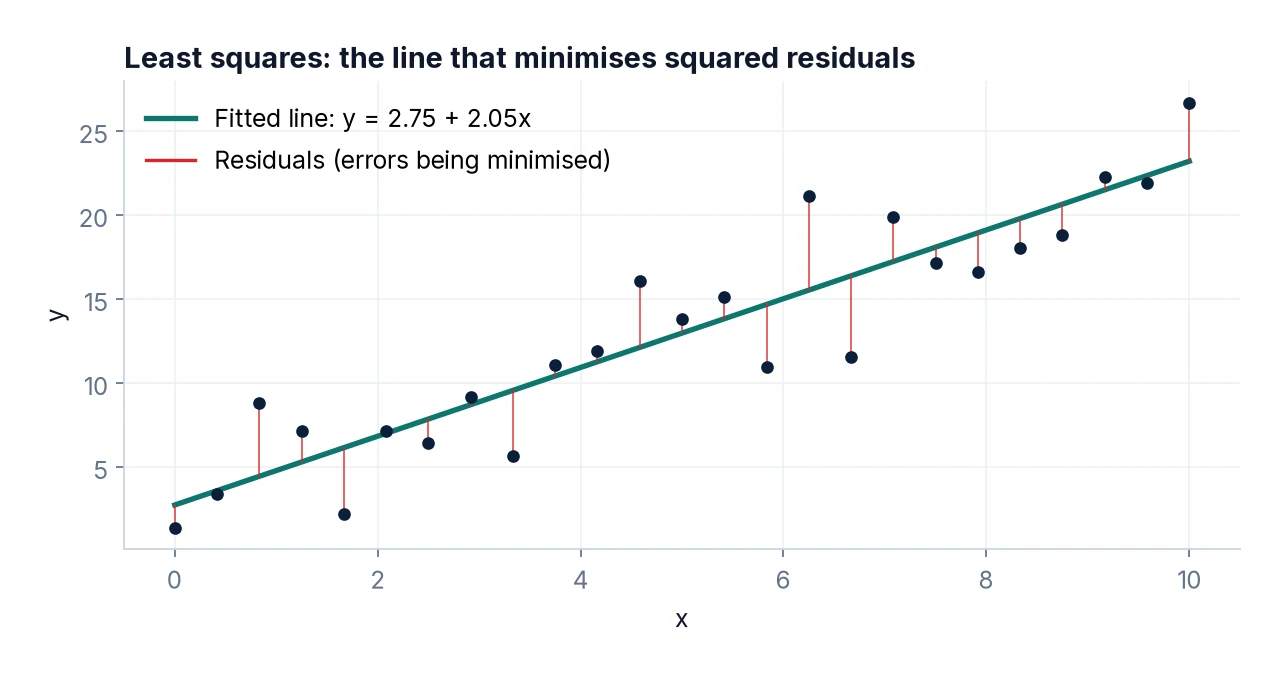
prediction = intercept + slope × feature

With several features, it fits one coefficient per feature:

prediction = b0 + b1×x1 + b2×x2 + ... + bn×xn

“Fitting” means choosing the coefficients that minimise the sum of squared differences between predictions and actual values. This is called ordinary least squares (OLS). Squaring means large errors are penalised heavily, which is worth remembering when your data has outliers.

Step 1: A simple example with known answers

To build intuition, generate data where we know the true relationship – say, delivery cost = £4 + £0.50 per kilometre, plus some random noise – and check that the model recovers it.

import numpy as np
import pandas as pd
from sklearn.linear_model import LinearRegression

rng = np.random.default_rng(42)
km = rng.uniform(1, 40, size=200)
cost = 4 + 0.5 * km + rng.normal(0, 1.5, size=200)

df = pd.DataFrame({"km": km, "cost": cost})
model = LinearRegression()
model.fit(df[["km"]], df["cost"])

print("Intercept:", round(model.intercept_, 2))
print("Slope:    ", round(model.coef_[0], 3))
print("Predicted cost for 10 km:", round(model.predict(pd.DataFrame({"km": [10]}))[0], 2))

The fitted slope comes out very close to the true 0.5 and the intercept is in the region of 4 – not exact, because of the random noise, but clearly recovering the real relationship. With more data or less noise, the estimates get closer still. Note the double brackets in df[["km"]]: scikit-learn expects the features as a two-dimensional table (rows × columns), even when there is only one column. Passing df["km"] gives the error “Expected 2D array, got 1D array instead”.

Step 2: Load a real dataset

We will use the diabetes dataset bundled with scikit-learn. It has 442 patients, ten baseline measurements (age, sex, BMI, blood pressure and six blood serum measurements) and a target that measures disease progression one year later. The features have already been centred and scaled by the dataset’s authors, which is why the values look small.

from sklearn.datasets import load_diabetes

X, y = load_diabetes(return_X_y=True, as_frame=True)
print(X.shape)
print(X.head())
print(y.describe())

Step 3: Split, train and predict

Always hold back data the model has not seen. If you are unsure why, read Train/Test Split Explained first.

from sklearn.model_selection import train_test_split

X_train, X_test, y_train, y_test = train_test_split(
    X, y, test_size=0.2, random_state=42)

reg = LinearRegression().fit(X_train, y_train)
y_pred = reg.predict(X_test)
print(y_pred[:5].round(1))
print(y_test.values[:5])

Step 4: Evaluate the model

Three metrics cover most needs:

• MAE (mean absolute error) – the average size of an error, in the target’s units. Easy to explain.
• RMSE (root mean squared error) – also in the target’s units, but punishes big errors more.
• R² – the proportion of variance in the target explained by the model. 1 is perfect; 0 is no better than always predicting the average; it can be negative for a model worse than that.

from sklearn.metrics import mean_absolute_error, mean_squared_error, r2_score

mae = mean_absolute_error(y_test, y_pred)
rmse = np.sqrt(mean_squared_error(y_test, y_pred))
r2 = r2_score(y_test, y_pred)
print(f"MAE:  {mae:.1f}")
print(f"RMSE: {rmse:.1f}")
print(f"R²:   {r2:.3f}")

# Baseline: always predict the training mean
baseline = np.full(len(y_test), y_train.mean())
print(f"Baseline MAE: {mean_absolute_error(y_test, baseline):.1f}")

On this split the model explains roughly half of the variance (R² about 0.45), and its MAE is well below that of the baseline. That is a real improvement, but far from perfect – typical of medical data, where much of the variation depends on factors not in the dataset. Always compare against a simple baseline: a metric on its own means little without context.

Step 5: Interpret the coefficients

Each coefficient tells you how much the prediction changes when that feature increases by one unit, holding the other features constant.

coefs = pd.Series(reg.coef_, index=X.columns).sort_values()
print(coefs.round(1))
print("Intercept:", round(reg.intercept_, 1))

Because these features were pre-scaled to similar ranges, the size of each coefficient gives a rough sense of its influence; BMI and one of the serum measurements (s5) have large positive coefficients, while s1 has a large negative one. Be careful with two things:

• Scale. If features are in different units (kilometres and pounds, say), raw coefficient sizes are not comparable. Standardise features first if you want to compare them.
• Correlated features. The serum measurements are correlated with each other, which can make individual coefficients unstable and even give them surprising signs – the large opposite-signed coefficients on s1 and s2 are a classic symptom. The predictions can still be good while the individual coefficients are hard to interpret.

And coefficients describe associations in this data, not cause and effect.

Step 6: Check the residuals

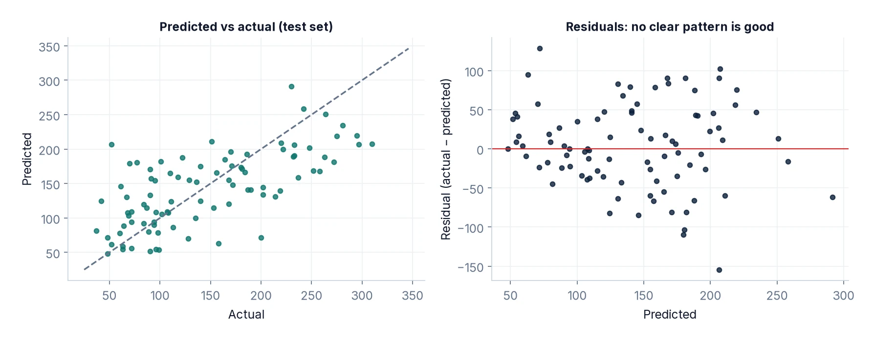
Residuals are the differences between actual and predicted values. Plotting them against predictions is the quickest way to spot problems:

import matplotlib
matplotlib.use("Agg")  # remove this line in a notebook
import matplotlib.pyplot as plt

residuals = y_test - y_pred
plt.scatter(y_pred, residuals, alpha=0.6)
plt.axhline(0, color="grey", linestyle="--")
plt.xlabel("Predicted value")
plt.ylabel("Residual (actual − predicted)")
plt.title("Residuals vs predictions")
plt.savefig("residuals.png", dpi=120, bbox_inches="tight")
print("Mean residual:", round(residuals.mean(), 2))

What you want to see is a shapeless cloud centred on zero. Warning signs include:

• A curve – the relationship is not linear. Try transforming features (for example a log or squared term) or a non-linear model.
• A funnel that widens – errors grow with the prediction. A log transform of the target often helps.
• A few extreme points – check them for data errors.

Step 7: Handle categorical features

Linear regression needs numbers. Categories such as region or product type must be converted, usually with one-hot encoding. A ColumnTransformer inside a Pipeline does this safely, learning the categories from training data only:

from sklearn.compose import ColumnTransformer
from sklearn.preprocessing import OneHotEncoder, StandardScaler
from sklearn.pipeline import Pipeline

houses = pd.DataFrame({
    "floor_area": rng.uniform(40, 200, 300),
    "bedrooms": rng.integers(1, 6, 300),
    "region": rng.choice(["North", "Midlands", "South"], 300),
})
uplift = houses["region"].map({"North": 0, "Midlands": 20000, "South": 60000})
houses["price"] = 50000 + 1500 * houses["floor_area"] + 8000 * houses["bedrooms"] + uplift \
                  + rng.normal(0, 15000, 300)

features = ["floor_area", "bedrooms", "region"]
pre = ColumnTransformer([
    ("num", StandardScaler(), ["floor_area", "bedrooms"]),
    ("cat", OneHotEncoder(handle_unknown="ignore", drop="first"), ["region"]),
])
pipe = Pipeline([("pre", pre), ("reg", LinearRegression())])

Xh_train, Xh_test, yh_train, yh_test = train_test_split(
    houses[features], houses["price"], test_size=0.2, random_state=0)
pipe.fit(Xh_train, yh_train)
print("R² on test:", round(pipe.score(Xh_test, yh_test), 3))

This is synthetic data built for illustration, so the high R² simply reflects how it was generated; real house prices are much noisier. The structure, however, is exactly what you would use on real data.

Common mistakes

• Evaluating on training data. Always use a held-out test set or cross-validation.
• Passing a 1D array as features. Use df[["col"]].
• Ignoring the baseline. An RMSE of 50 is good or bad only relative to a naive prediction.
• Treating coefficients as causal effects.
• Label-encoding categories as 1, 2, 3, which implies an order and equal spacing that does not exist. Use one-hot encoding.
• Extrapolating. A model trained on houses of 40–200 m² says little about a 1,000 m² mansion.
• Skipping residual checks. A decent R² can hide a clearly non-linear pattern.

FAQ

Do I need to scale features for linear regression?

Plain OLS gives the same predictions with or without scaling. Scaling matters for regularised versions (Ridge, Lasso) and for comparing coefficients.

What are Ridge and Lasso?

Variants that add a penalty on large coefficients, which reduces overfitting and helps with correlated features. Lasso can shrink some coefficients to exactly zero, acting as feature selection. Both are in sklearn.linear_model.

How do I get p-values?

scikit-learn focuses on prediction and does not report them. For statistical inference, use the statsmodels library’s OLS.

What if my target is a category, not a number?

Use a classification model such as logistic regression.

Next steps

Get more reliable performance estimates with cross-validation, improve your inputs with feature engineering, and move on to classification with logistic regression and classification metrics. If your data needs tidying first, see Cleaning Messy Data with Pandas.