Classification Metrics Explained: Accuracy, Precision, Recall, F1

You have trained a classifier and it reports 95% accuracy. Is that good? It depends entirely on the problem. If only 5% of cases are positive, a model that always predicts “negative” also scores 95% – while being completely useless. Accuracy alone can hide that.

This tutorial explains the metrics you need to judge a classification model properly: the confusion matrix, accuracy, precision, recall, F1, and the decision threshold that links them. We will calculate everything by hand on a tiny example first, then with scikit-learn on a real dataset, so you understand both what the numbers mean and how to produce them.

A hypothetical example to build intuition

Imagine a fraud model tested on 1,000 card transactions, of which 10 are actually fraudulent. (These numbers are invented purely for illustration.) A model that labels every transaction as genuine gets 990 right – 99% accuracy – and catches zero fraud. That is the “accuracy paradox”, and it is why we need metrics that look at each class separately.

Step 1: The confusion matrix

For a binary problem, every prediction falls into one of four boxes. We call the class we care about detecting the positive class (fraud, disease, churn).

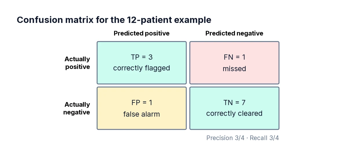
• True Positive (TP) – predicted positive, actually positive.
• False Positive (FP) – predicted positive, actually negative (a false alarm).
• True Negative (TN) – predicted negative, actually negative.
• False Negative (FN) – predicted negative, actually positive (a miss).

Let us compute these for twelve made-up predictions:

import numpy as np
from sklearn.metrics import confusion_matrix

y_true = np.array([1, 1, 1, 1, 0, 0, 0, 0, 0, 0, 0, 0])
y_pred = np.array([1, 1, 1, 0, 1, 0, 0, 0, 0, 0, 0, 0])

tn, fp, fn, tp = confusion_matrix(y_true, y_pred).ravel()
print(f"TP={tp}  FP={fp}  TN={tn}  FN={fn}")

Output: TP=3, FP=1, TN=7, FN=1. There were four real positives; the model caught three and missed one, and it raised one false alarm.

Note that scikit-learn’s confusion matrix puts actual classes in rows and predicted classes in columns, ordered by label (0 then 1). Some textbooks lay it out the other way round, so always check the orientation.

Step 2: Accuracy

accuracy = (TP + TN) / total

Here: (3 + 7) / 12 ≈ 0.833. Accuracy is fine when classes are roughly balanced and both kinds of error cost about the same. Otherwise, it misleads.

Step 3: Precision – “when it says yes, how often is it right?”

precision = TP / (TP + FP)

Here: 3 / 4 = 0.75. Of the four cases flagged as positive, three really were. High precision means few false alarms. Precision matters most when acting on a false positive is costly: blocking a genuine customer’s card, sending an expensive retention offer, or flagging a legitimate email as spam.

Step 4: Recall – “of all the real positives, how many did it find?”

recall = TP / (TP + FN)

Here: 3 / 4 = 0.75. The model found three of the four real positives. Recall is also called sensitivity or the true positive rate. It matters most when missing a positive is costly: an undetected disease, a fraudulent transaction that goes through, a safety defect.

Step 5: F1 score – balancing the two

F1 = 2 × precision × recall / (precision + recall)

F1 is the harmonic mean of precision and recall. Unlike a simple average, it is dragged down sharply if either one is low, so a model cannot score well by maximising one and ignoring the other. Here both are 0.75, so F1 is 0.75.

Let us confirm all of these with scikit-learn:

from sklearn.metrics import accuracy_score, precision_score, recall_score, f1_score

print("Accuracy :", round(accuracy_score(y_true, y_pred), 3))
print("Precision:", round(precision_score(y_true, y_pred), 3))
print("Recall   :", round(recall_score(y_true, y_pred), 3))
print("F1       :", round(f1_score(y_true, y_pred), 3))

Step 6: A real model

Now let us apply these metrics to a real classifier using the breast cancer dataset bundled with scikit-learn. In this dataset, label 0 means malignant and 1 means benign. Since malignant is the class we want to detect, we flip the labels so that 1 = malignant. Getting the positive class right is essential: precision and recall are always calculated for the positive class.

from sklearn.datasets import load_breast_cancer
from sklearn.model_selection import train_test_split
from sklearn.pipeline import make_pipeline
from sklearn.preprocessing import StandardScaler
from sklearn.linear_model import LogisticRegression
from sklearn.metrics import classification_report

X, y = load_breast_cancer(return_X_y=True)
y = 1 - y   # now 1 = malignant (positive class)

X_train, X_test, y_train, y_test = train_test_split(
    X, y, test_size=0.25, random_state=42, stratify=y)

model = make_pipeline(StandardScaler(), LogisticRegression(max_iter=1000))
model.fit(X_train, y_train)
pred = model.predict(X_test)

print(confusion_matrix(y_test, pred))
print(classification_report(y_test, pred, target_names=["benign", "malignant"], digits=3))

classification_report prints precision, recall and F1 for each class, plus the number of cases (“support”). Read the row for the class you care about. The report also shows two averages across classes: the macro average treats each class equally, while the weighted average weights by support, so it is dominated by the larger class.

The split, scaling and pipeline here follow the approach in Train/Test Split Explained, and the model itself is explained in Logistic Regression in Python.

Step 7: The threshold controls the trade-off

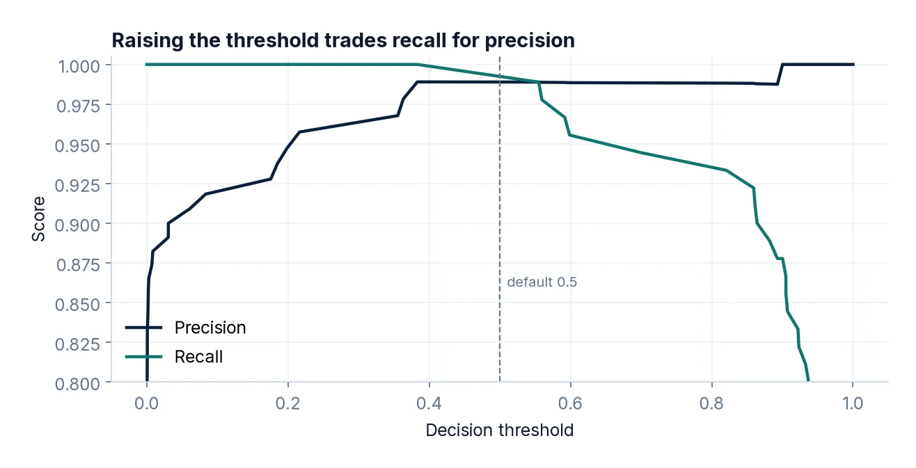
Most classifiers output a probability, and predict() simply applies a threshold of 0.5. Change the threshold and you trade precision for recall. Lowering it flags more cases as positive: recall goes up, precision usually goes down.

proba = model.predict_proba(X_test)[:, 1]   # probability of malignant

for threshold in [0.2, 0.35, 0.5, 0.65, 0.8]:
    p = (proba >= threshold).astype(int)
    print(f"threshold={threshold:.2f}  "
          f"precision={precision_score(y_test, p):.3f}  "
          f"recall={recall_score(y_test, p):.3f}  "
          f"FN={((p == 0) & (y_test == 1)).sum()}")

Run this and you will see recall rise as the threshold falls, with the number of missed malignant cases (FN) shrinking, at the cost of more false alarms. For a screening tool, a low threshold may well be appropriate, because a false alarm leads to a further test while a miss could be serious. The right threshold is a business or clinical decision, not a statistical one; your job is to make the trade-off visible.

Step 8: Threshold-free metrics

To compare models without choosing a threshold, use metrics computed from the probabilities across all thresholds:

• ROC AUC – the probability that the model ranks a random positive above a random negative. 0.5 is random guessing, 1.0 is perfect.
• Average precision (PR AUC) – summarises the precision–recall curve. It is more informative than ROC AUC when positives are rare, because ROC AUC can look high even when precision is poor.

from sklearn.metrics import roc_auc_score, average_precision_score

print("ROC AUC:          ", round(roc_auc_score(y_test, proba), 3))
print("Average precision:", round(average_precision_score(y_test, proba), 3))

Which metric should you use?

• Balanced classes, similar error costs: accuracy is fine; report F1 too.
• False positives are expensive: focus on precision.
• False negatives are expensive: focus on recall.
• Both matter and classes are imbalanced: F1 and average precision.
• Comparing models before choosing a threshold: ROC AUC or average precision.

Whatever you choose, show the confusion matrix too. Stakeholders understand “caught 49 of the 53 malignant cases, with 1 false alarm” (the result from the 0.5 threshold above) far better than “F1 = 0.94”.

Common mistakes

• Reporting only accuracy on imbalanced data.
• Getting the positive class wrong. scikit-learn treats label 1 as positive by default. Check, or set pos_label.
• Misreading the confusion matrix orientation.
• Choosing the threshold on the test set. Tune it on validation data, then confirm on the test set.
• Quoting weighted averages that hide poor performance on a small but important class.
• Ignoring the cost of errors. Metrics are only meaningful in the context of what each mistake costs.

FAQ

What is a good F1 score?

There is no universal threshold. Compare against a baseline (such as always predicting the majority class) and against what is useful in practice.

What is specificity?

The true negative rate: TN / (TN + FP). It is the “recall” of the negative class and is common in medical contexts alongside sensitivity.

How do these metrics work with more than two classes?

Precision, recall and F1 are calculated per class (treating each as positive in turn) and then averaged – macro, weighted or micro. classification_report shows them all.

Should I use cross-validation for metrics?

Yes, especially with small datasets. See Cross-Validation: A Practical Guide.

Next steps

Build the classifier itself in Logistic Regression in Python, get more stable estimates with cross-validation, and improve the inputs with feature engineering. For predicting numbers rather than classes, see Linear Regression in Python.